Reduction of Low-Frequency Vessel Noise in Monterey Bay National Marine Sanctuary During the COVID-19 Pandemic

Introduction

Shipping is a dominant source of low-frequency anthropogenic noise in the ocean (Wenz, 1962; Hildebrand, 2009; Southall et al., 2017). Research using passive acoustic monitoring off California has identified increasing trends in low-frequency ocean noise of ∼3 dB per decade over ∼40 years, attributed to increases in commercial ship traffic (Andrew et al., 2002; McDonald et al., 2006), though trends may have changed differently in different areas since the 1990s (Andrew et al., 2011). Reduction of shipping noise off California has been observed over shorter time scales (<1 year) as a result of economic recession and associated reduction of maritime shipping activity, as well as regulatory changes that affected routing (McKenna et al., 2012).

Among the many human activities curtailed by the COVID-19 pandemic during 2020 was maritime shipping, resulting in reduced low-frequency ocean noise levels documented in some areas (Thomson and Barclay, 2020). This major change in global economic activity enables a rare opportunity to quantify the relationship between vessel activity and soundscape conditions in biologically important marine habitats. The habitat that is the focus of this study is centered within Monterey Bay National Marine Sanctuary (MBNMS), which extends ∼ 300 km along the central California coast and includes a wide variety of rich habitats, including an offshore biodiversity hotspot–Davidson Seamount (Figure 1). Years of continuous sound recording within MBNMS (Ryan et al., 2016), enabled by the Monterey Accelerated Research System (MARS) cabled observatory (Figure 1), support examination of 2020 ambient noise levels relative to those existing in previous years.

FIGURE 1

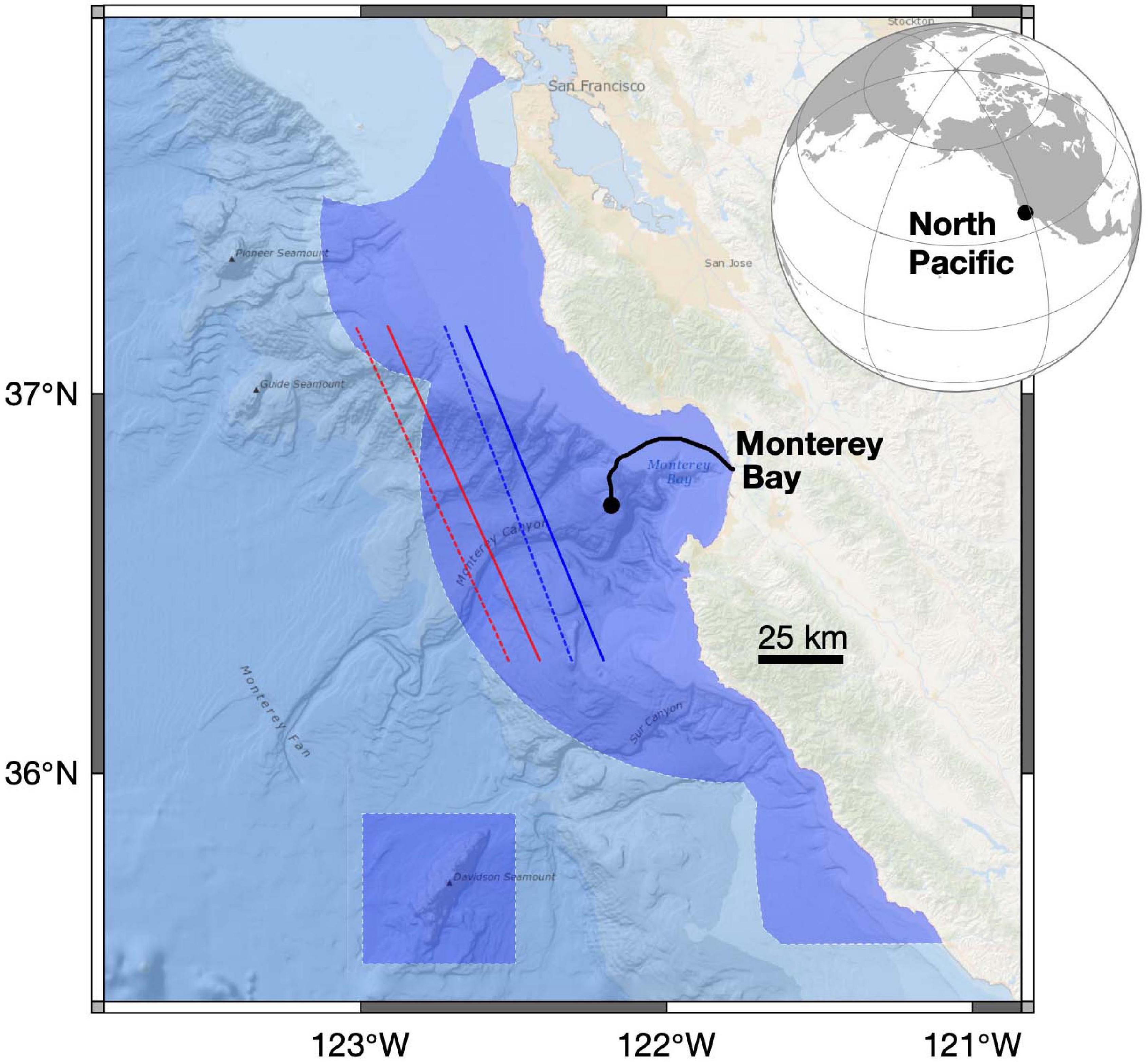
Figure 1. The study region along the eastern margin of the North Pacific. Blue shaded regions define the Monterey Bay National Marine Sanctuary, which includes a region adjacent to the California coast centered on Monterey Bay and an offshore region around Davidson Seamount. The hydrophone is connected to the Monterey Accelerated Research System (MARS) cabled observatory (black line and circle; main node at 36.713°N, 122.186°W, 891 m depth). Blue and red lines define recommended tracks for northbound (solid) and southbound (dashed) shipping traffic for vessels 300 gross tons and above; red lines are for vessels carrying hazardous cargo in bulk or crude oil.

Located within the highly productive California Current Large Marine Ecosystem (Ekstrom, 2009), and centered over the largest submarine canyon off the North American west coast, MBNMS is an important habitat for abundant and diverse marine life, including at least 34 mammal species (NOAA, 2017). MBNMS is considered to be a biologically important area (BIA) for multiple species of baleen whales (Calambokidis et al., 2015), whose use of low-frequency sound for communication makes them relatively susceptible to interference from low-frequency anthropogenic noise. Particularly soniferous species of baleen whales that inhabit MBNMS include blue, fin, and humpback (Figure 2). The region is also an important habitat for gray whales that migrate along the eastern margin of the North Pacific, moving through MBNMS where their calves are susceptible to predation by orcas (Goley and Straley, 1994). In their NE Pacific breeding habitat, gray whales have exhibited increased vocalization rates and source levels in response to vessel noise (Dahlheim and Castellote, 2016), a response that could influence acoustic detection by orcas and associated predation risk in MBNMS if exhibited during northward migration.

FIGURE 2

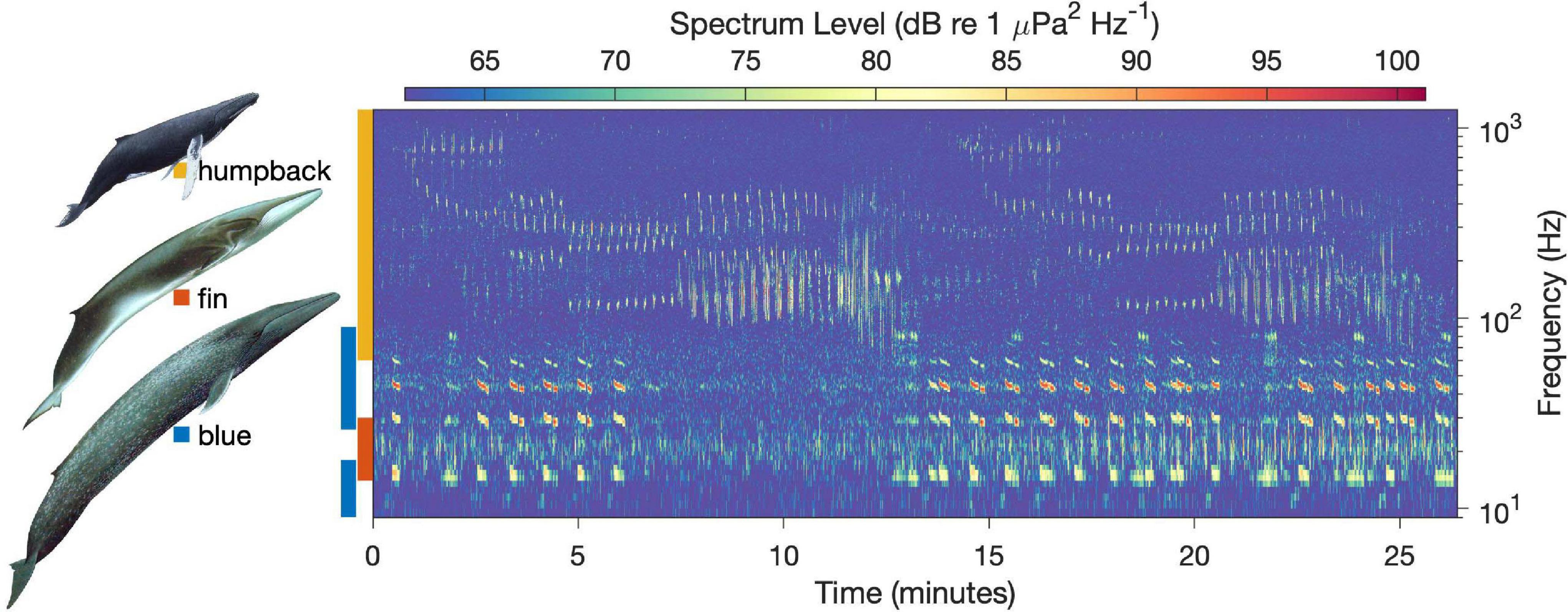
Figure 2. Simultaneous song from three baleen whale species recorded in Monterey Bay National Marine Sanctuary. Spectrogram calculation used 12.8 kHz data (decimated from 256 kHz), 12,800 pt. FFT, Hanning window, 50% overlap; start time is 10-Jan-2017 13:33 UTC. Colored bars along the vertical axis define the approximate frequency ranges used by each species. Humpback song spans the greatest frequency range and is the most complex, with two full songs represented (beginning at ∼1 and 15 min). Blue whale song includes three call types: A calls—pulse-trains centered near 80 Hz, B calls—the loudest calls produced with fundamental frequency centered near 14.5 Hz and harmonics centered near 29, 43.5, and 58 Hz, and C calls—the subtlest of the three, centered near 11 Hz. Fin whale song is the simplest, consisting of brief (∼ 1 s) pulses that are modulated in frequency and variably paired in singlets, doublets, and triplets (Helble et al., 2020). Baleen whale song occurrence within the foraging habitat of MBNMS spans 7–9 months of the year, depending on the species (Ryan et al., 2019; Oestreich et al., 2020). Whale artist: Larry Foster.

Protection of acoustic habitat in the ocean is an ongoing and rising priority (Southall et al., 2009; Hatch et al., 2016; Chou et al., 2021; Duarte et al., 2021), and passive acoustic monitoring has become integral to the management of marine protected areas (Gottesman et al., 2020; Kline et al., 2020). The ways that anthropogenic noise can affect marine mammals include interference with communication (masking), behavioral disturbance such as avoidance of key habitat areas essential to fitness and survival, induction of chronic or acute stress, and in severe cases physiological damage (Hatch et al., 2008, 2012; Rolland et al., 2012; Gedamke et al., 2016; Erbe et al., 2019; Simonis et al., 2020a). Within MBNMS, the threat posed by fishery explosions to acoustically sensitive harbor porpoise has been considered (Simonis et al., 2020b). In this contribution, we examine changes in ocean noise within MBNMS resulting from pandemic-induced reductions in maritime shipping activity. We consider how this unanticipated change provides a window into noise as a pollutant that can be managed within a multi-use ocean environment to better protect biologically important habitats and the species that inhabit them.

Materials and Methods

Acoustic Data and Analyses

Acoustic recordings were acquired through the Monterey Accelerated Research System (MARS) cabled observatory, located in the center of MBNMS (Figure 1). Since 28 July 2015, MARS has supported nearly continuous recording at a sample rate of 256 kHz using an Ocean Sonics icListen HF—an omnidirectional hydrophone with a bandwidth of 10 Hz–200 kHz. Data stream directly to the Ocean Sonics Lucy software for shore-side recording. Because the potential impacts of the COVID-19 pandemic on U.S. shipping traffic began during the first few months of 2020, we examine January through July recordings from 2020 in relation to the same months of the preceding 2 years. During this study period, recording temporal coverage was 96.4%. This entire period was recorded by one continuously deployed hydrophone that exhibited no long-term trends in low-frequency noise, thus supporting effective comparison across years.

The shipping noise metric computed was mean-square sound pressure spectral density, ISO 18405 3.1.3.13 (ISO, 2017), for the one-third octave band centered at 63 Hz (Band 18, Dekeling et al., 2014). Power spectral density (PSD) was computed from 2 kHz data at resolutions of 1 s and 1 Hz using Welch’s method in MATLAB (pwelch, FFT length = 2,000 points, Hanning window length = 2,000 points). PSD was averaged for the 63 Hz one-third octave band, and median (L50) values were extracted for the temporal observation window (IQOE, 2019) of 1 min. Calibrated spectrum levels were computed by subtracting the manufacturer-measured hydrophone sensitivity for the low-frequency range (−177.9 dB re 1 V/μPa at 250 Hz). The icListen is a digital hydrophone in which there is no separation between the sensor element, filters, amplifier, and analog-to-digital converter. The internal amplifier gain is included in the reported sensitivity. Although independent calibration in the focal frequency band is ideal, this is not a concern for this analysis, which applies relative comparison of monthly ambient noise statistics. Monthly statistics, including geometric mean and exceedance levels at 10, 25, 50, 75, and 90%, were examined to quantify changes during 2020 and to compare 2020 with the preceding 2 years. For the year-to-year comparisons of monthly data, we applied analysis of variance and Tukey Honest Significant Differences (HSD) multiple comparison tests using the stats package in R (Version 3.6).

The acoustic data processing methods described above effectively removed two signals that would otherwise confuse analysis of shipping noise. The first signal is biophony from blue whales, specifically the fourth harmonic of the song-associated B call. The strong signal of this source in the 63 Hz one-third octave band is effectively eliminated by the 1-min L50 (Figure 3A). During fall months when blue whale song rises to peak occurrence (Oestreich et al., 2020), chorusing of blue whales is more probable, and this method may be less effective. However, it is reliable for the winter, spring, and summer months of our study. The second signal is not part of the soundscape, but instead caused by mechanical disturbance of the hydrophone. These extreme, transient broadband signals sound like direct contact between animals and the hydrophone (bio-abrasion). Because these transient signals do not occupy a large percentage of the time windows within which they occur, the 1-min L50 effectively eliminates this signal from monthly statistical descriptions (Figure 3B).

FIGURE 3

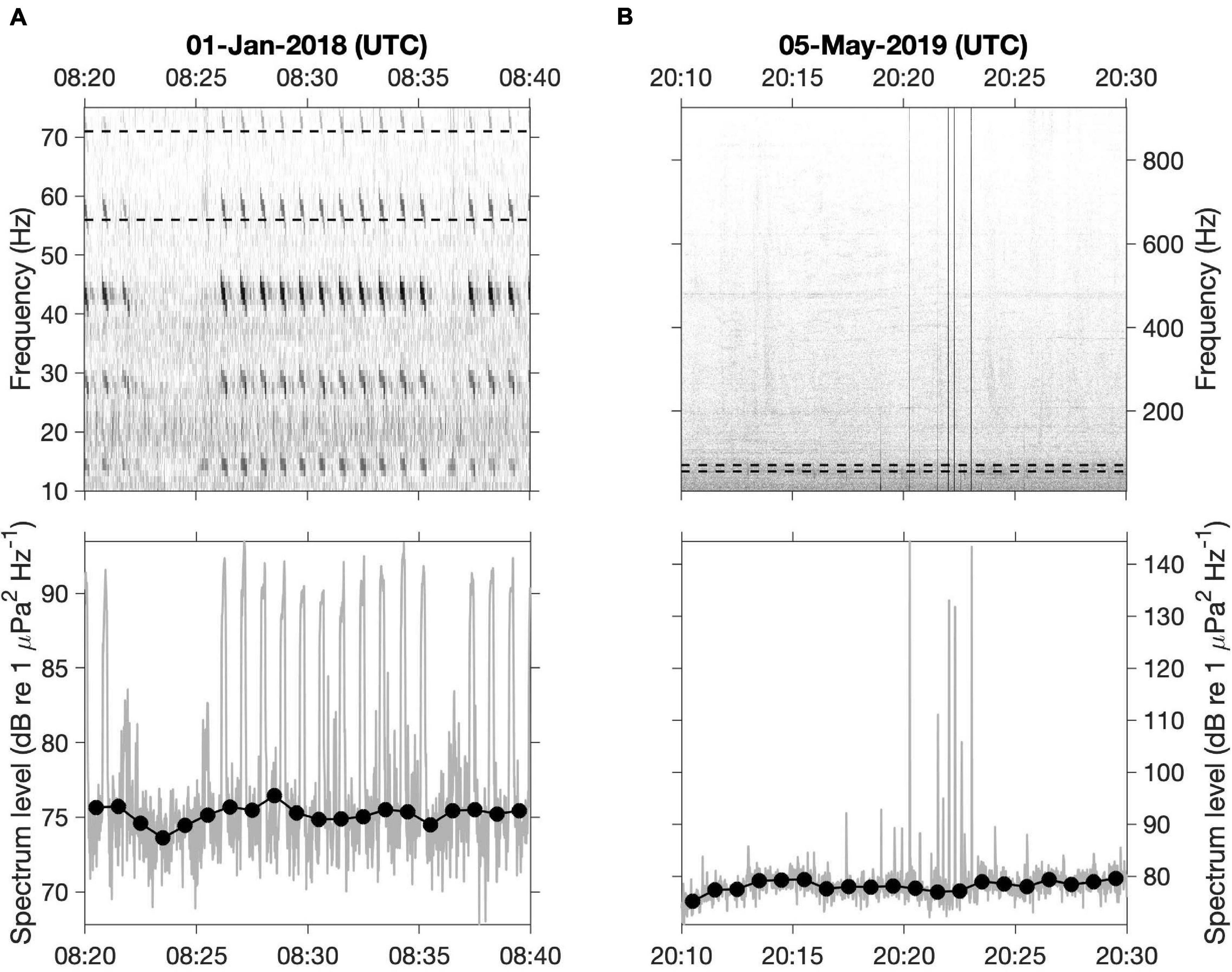
Figure 3. Non-shipping signals in the focal frequency band. Focal signals are (A) the fourth harmonic of the blue whale B call, and (B) bio-abrasion (mechanical disturbance of the recorder by an animal). Spectrograms (top) were computed using 2 kHz data (decimated from 256 kHz), 2,000 pt. FFT, Hanning window, no overlap; the 63-Hz one-third octave band is represented by dashed lines. Spectrum levels within the focal frequency band (bottom) are represented for 1-s resolution (gray) and 1-min L50 (black).

Economic Data and Analyses

Data on marine vessels entering and leaving U.S. ports are collected by Customs and Border Protection and provided as a weekly dataset to the Maritime Administration. Each record includes the date and time of entry or clearance, the name of the port, and information of the vessel such as its tonnage and type. For the period of the acoustic data analyses, January through July of 2018–2020, the Maritime Administration aggregated the data on vessel entries into ports in California and calculated monthly summary statistics including the total number of port calls and the total gross tonnage by port. Most of the reported gross tonnage (91%) was for cargo vessel types (container, tanker, roll-on/roll-off, dry bulk, general cargo, barge) while the remaining 9% comprised passenger vessels.

Automatic Identification System Vessel Tracking Data and Analyses

Automatic Identification System (AIS) data for Monterey Bay and the surrounding region were acquired from the U.S. Coast Guard, covering the time period of the acoustic data analyses, January through July of 2018–2020. The data are summaries of average positions every 5 min for every vessel recorded, and ancillary data for each vessel. AIS data covering a large domain (35–38.5°N, 124.5–120.5°W) were acquired, including the intensive shipping traffic associated with ports in San Francisco Bay. Two categories of AIS records were removed prior to analysis. Records having positions over land or within San Francisco Bay were removed using the inpolygon function of the pracma package for R (Version 3.6.3) with a land polygon mask defined by full-resolution GSHHS coastline data. Redundant records were removed by requiring that a vessel, identified by its Maritime Mobile Service Identity (MMSI) number, be represented only once in each 5-min data summary. Vessel length was computed by adding the AIS data fields that quantify the distances between the AIS transmitter and the vessel’s bow and stern. This length was used to confirm that records in the category of other types of ship represented large vessels of interest in this study (USCG, 2021; ship and cargo type beginning with 9).

A proxy for potential low-frequency noise from large vessels was derived from a vessel noise model and AIS vessel presence records weighted by two scaling factors. The first was vessel speed. A statistical model developed using nearly 600 examples of recorded container vessel transits showed that vessel speed had the greatest predictive power for noise across the full frequency range examined, 20–1,000 Hz (McKenna et al., 2013). According to this model, vessel noise source level (SL) is a quasi-exponential function of vessel speed. In the present study, the duration of each record of vessel presence (5 min) was weighted based on vessel speed using the published model function for the octave band centered at 63 Hz. Records having unreasonably high vessel speeds (>25 knots, 0.04% of records) were excluded. The second factor used modeled acoustic transmission loss (TL) at 63 Hz (section “Acoustic Modeling”). Specifically, the weighting factor = 10^{[–(TL–TLmin)/10]}, scaled such that the minimum TL within the model domain (near the hydrophone) was assigned a weighting value of 1 and all other TL values were assigned weighting values below 1. Specification of this weighting factor is based on the definition TL = 10log₁₀(linear-scale transmission loss).

Relationships Between Vessel Activity and Low-Frequency Noise

Because monthly geometric means of ambient noise levels consistently track monthly changes quantified by exceedance levels, unlike arithmetic means, we use monthly geometric means in examining relationships between ambient noise and vessel activity. Relationships were examined for: (1) 2020 only, to consider causality of variation during the year that exhibited reduced noise, and (2) 2018–2020, to consider the strength of relationships within the full data set. These analyses were applied to examining relationships between the ambient noise metric and each shipping activity metric separately (derived from statewide port data and regional AIS data), as well as both shipping activity metrics together. Linear regression was conducted on the noise spectrum level (in dB) as a function of the logarithm of shipping activity, so that both the abscissa and the ordinate were on logarithmic scales. All statistical analyses were conducted in R, version 3.6. Correlations and their significance were examined using cor.test from the stats package. Linear models were fitted using lm from the stats package. Generalized additive models (GAMs) were fitted using gam from the mgcv (Mixed GAM Computation Vehicle with Automatic Smoothness Estimation) package. GAM modeling could be applied only to the full time series because input of 2020 data only would produce a smoothing term having fewer unique covariate combinations than the specified maximum degrees of freedom. Therefore, adjusted r²-values are from lm for 2020 data only, and from gam for 2018–2020 data. For GAM results we report the smoothing parameter estimation method (REML) and the effective degrees of freedom (EDF) (Zuur and Ieno, 2016), as well as the significance of the smoothing term.

Acoustic Modeling

Acoustic modeling was applied for two purposes. The first was to provide context for the recording site on the continental slope, surrounded by complex bathymetry, thereby explaining the typical pattern of noise received from large vessels transiting in the offshore shipping lanes. Using the BELLHOP model (Porter, 2011) we produced eigenray plots showing the rays that connect the receiver to vessels transiting in the shipping lanes. Eigenrays were examined for a series of bearing angles relative to the receiver, covering the full directional range spanned by the spatial relationship between the receiver and the shipping lanes. The nature and number of boundary interactions for each bearing were evaluated to characterize the directional range from which shipping noise can effectively reach the receiver. To consider the potential for distant shipping noise to reach the receiver via the SOFAR channel, ray tracing was modeled for the bearing of 242°, near the closest point of approach (CPA) within historical shipping lanes. Ray tracing shows the general pattern that sound energy originating from anywhere in the water column will arrive at the MARS receiver. Interaction with the surface and bottom boundaries results in significant energy loss from scattering and absorption, particularly at the ocean bottom.

The second purpose was to quantify acoustic transmission loss, as a basis for weighting AIS vessel records. This application used a wave-theory parabolic equation model that accounts for absorption in both the water column and the bottom, scattering in the water column and at the surface and bottom, geometric spreading (spherical and cylindrical), refraction, and diffraction (Collins, 1993). Source depth was specified as 6 m, and source frequency was specified as 63 Hz to be consistent with the shipping noise metric. The model domain extended 165 km from the receiver. Specification of regional ocean temperature and salinity was based on the January climatology from the US Navy Generalized Digital Environmental Model (GDEM). Bathymetry was specified at 250 m resolution.

Results

Acoustical Site Description

Typical attributes of low-frequency vessel noise received at the recording site are represented by a southbound transit of a large (332 m LOA) container vessel traveling at high speed (∼21 knots) in the lane second nearest to the recording site (Figures 1, 4). The first typical attribute is strong signal up to ∼100 Hz. The 63 Hz one-third octave band (overlaid in Figure 4) is effective for quantifying shipping noise at this location. The second typical attribute is indicated by the triangle and square markers within the spectrogram and inset reference map (Figure 4), which identify the steep rise and fall of received noise at specific points along the track. Results from the acoustic ray tracing model explain how the complex bathymetry of the continental shelf and slope surrounding the recording site (Figure 1) cause this attribute (Figure 5). Steep rise of noise for this southbound transit occurred when the ship crossed the continental shelf break, moving from shallow to deep water (triangles in Figures 4, 5A). North of this location, strong transmission loss results from many bottom reflections, particularly over the shelf (Figures 5B,C, 330°). The number of reflections and associated levels of transmission loss decrease as the ship moves over deeper water, to a minimum at CPA (Figures 5B,C, 242°). After moving south of CPA, the increased received levels (after ∼ 18:10 in Figure 4) are presumably due to the stern-facing attitude of the vessel relative to the receiver. As the ship passed Sur Ridge on the continental slope, received levels dropped steeply (squares in Figures 4, 5A). This was also caused by an increased number of bottom reflections due to the influence of the ridge on the ray paths (Figures 5B,C, 170°).

FIGURE 4

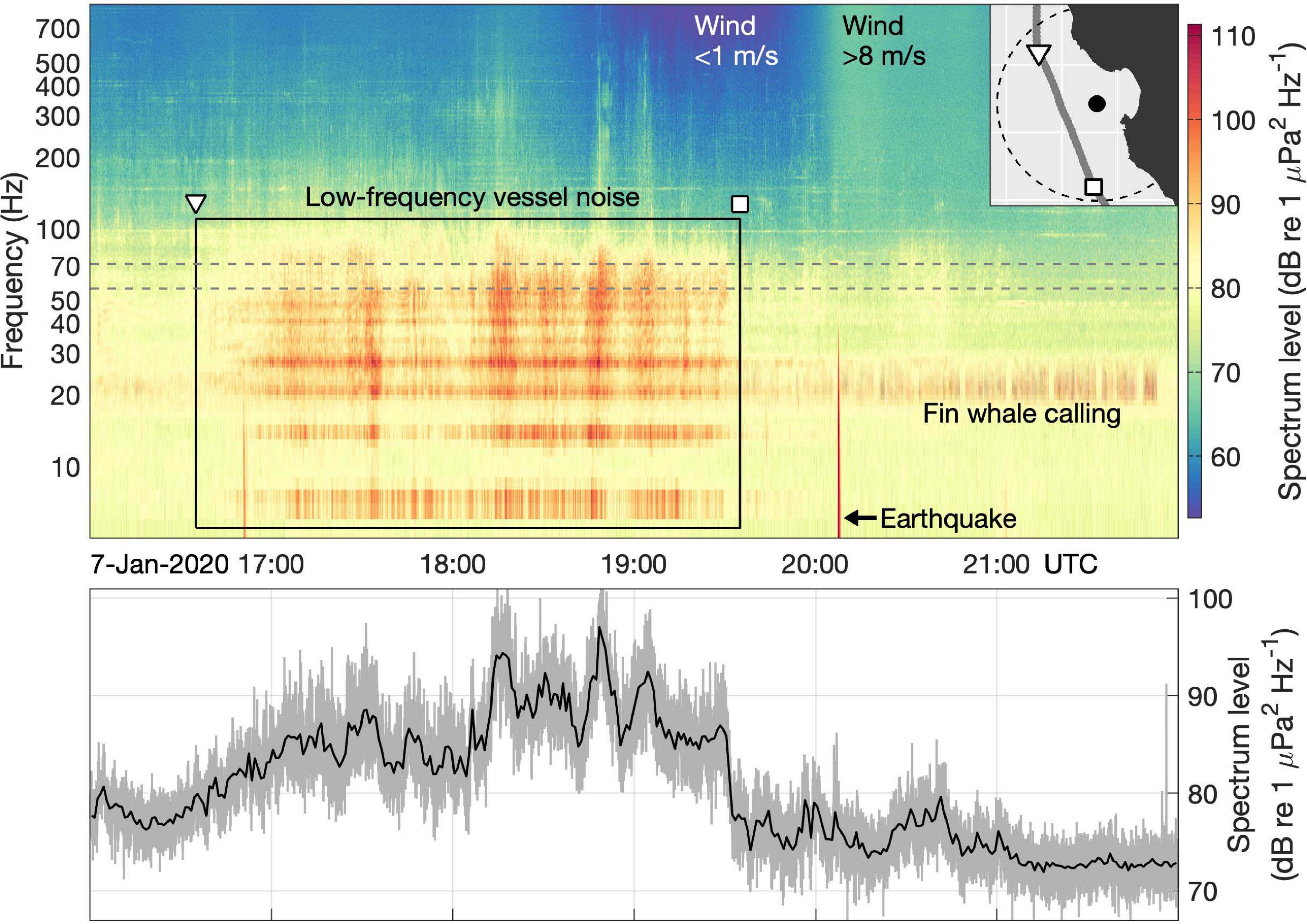
Figure 4. Low-frequency vessel noise within the greater soundscape at MARS. Spectrogram calculation used 2 kHz data (decimated from 256 kHz), 2,000 pt. FFT, Hanning window, no overlap. The box bounds temporal and frequency limits of the strongest signal from a southbound transit of the container vessel MSC SILVANA (IMO: 9309459; length overall 332 m). A portion of the vessel track is shown in the inset map, with time markers corresponding to those in the spectrogram (triangle, square); vessel speed was steady at 21.4 ± 0.16 knots during this portion of the transit. The black dashed line in the inset map defines an 80 km radius from MARS for scale reference. Other identifiable sounds include biological (fin whale calling) and geophysical (wind, earthquake). The fin whale calls are series of ∼ 1 s pulses with peak energy near 20 Hz. The increase in spectrum levels above ∼150 Hz beginning near hour 20 followed a rapid increase in wind speeds from < 1 m/s to > 8 m/s (measured at NDBC Station 46042, located 20.6 km NW of MARS). The dashed gray lines define the frequency band used to quantify shipping noise from the recording time series, the one-third octave band centered at 63 Hz. The lower panel represents spectrum levels for this focal frequency band at 1-s resolution (gray) and 1-min L50 (black).

FIGURE 5

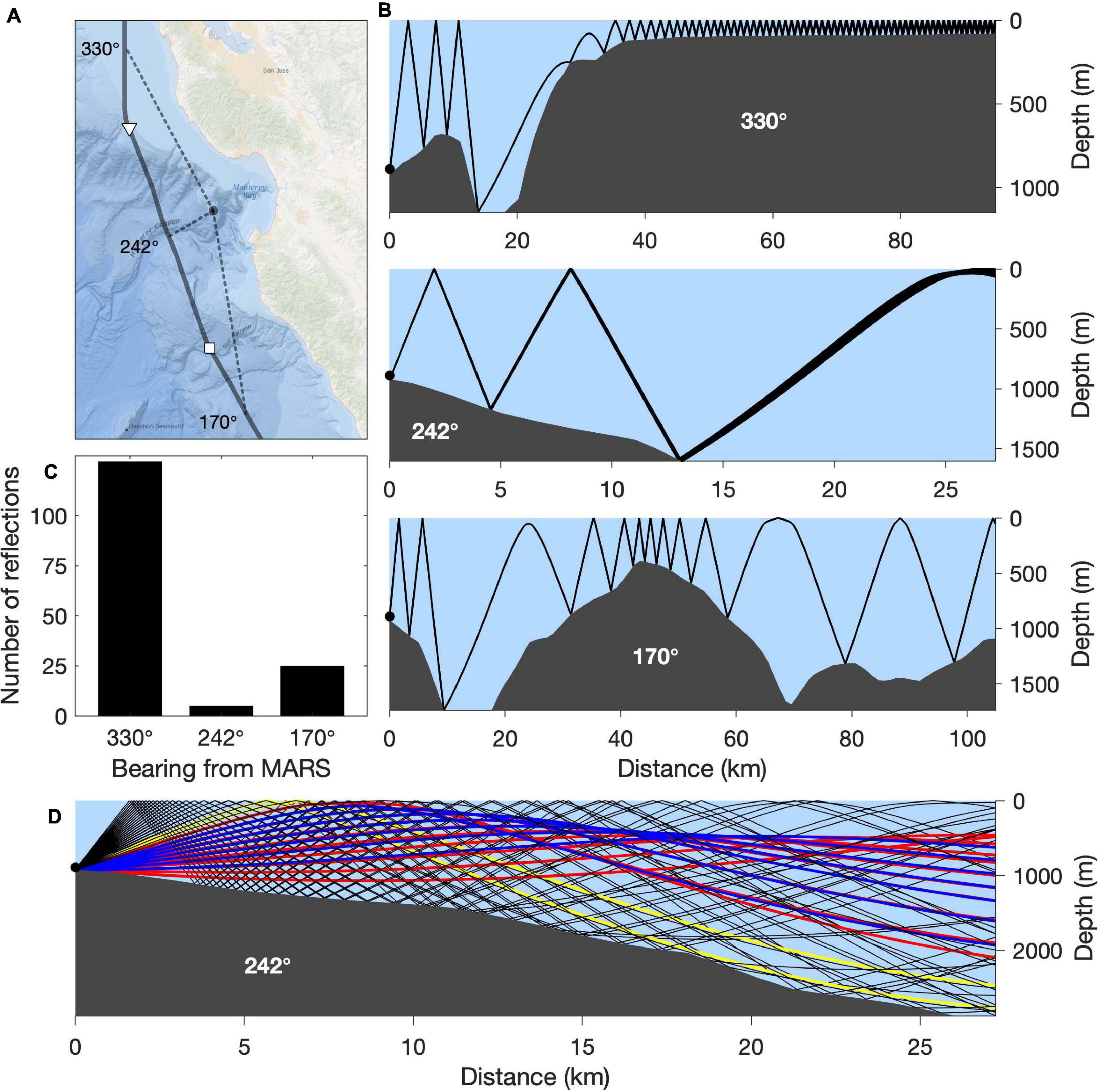
Figure 5. Acoustical characterization of the recording site. (A) Map showing the track of the MSC SILVANA (as in Figure 4). (B) Eigenrays between vessel source and MARS receiver computed using the BELLHOP model for the bearings identified in (A). (C) Total number of bottom and surface reflections for paths represented in (B). (D) Ray trace results for the 242° bearing. Black lines represent ray paths with multiple boundary interactions (high loss). Yellow lines represent paths that have only one surface reflection (small loss, particularly on calm days). Blue lines represent paths with only one bottom bounce, very near the receiver. Red lines represent paths with no boundary interaction over the range shown. The blue and red paths are in the SOFAR channel.

Because the recording site is within the depth range of the SOFAR channel, it is also important to consider the potential for distant shipping noise to reach the recorder via transmission within the SOFAR channel. Here again, bathymetry of the region surrounding the recording site is a primary determinant. Because ocean margin shipping lanes north and south of the recording site are bathymetrically blocked, the only directional range over which shipping noise could originate to reach the recording site via the SOFAR channel is offshore (∼ 180–300°). Results of the ray tracing model show that direct path sound energy from the SOFAR channel (red and blue eigenrays in Figure 5D) would have to originate from ∼ 500 m, well below the depth of vessel noise sources near the surface. Further, this directional range opens to low levels of vessel traffic beyond the shipping lanes (section “Relationship Between Low-Frequency Noise and Large-Vessel Activity”) and the full expanse of the North Pacific between the recorder and shipping activity of the western Pacific. Therefore, we conclude that our vessel noise metric effectively represents regional shipping activity, and that it is representative of what animals would be exposed to if located near our recording site (Figure 4).

FIGURE 6

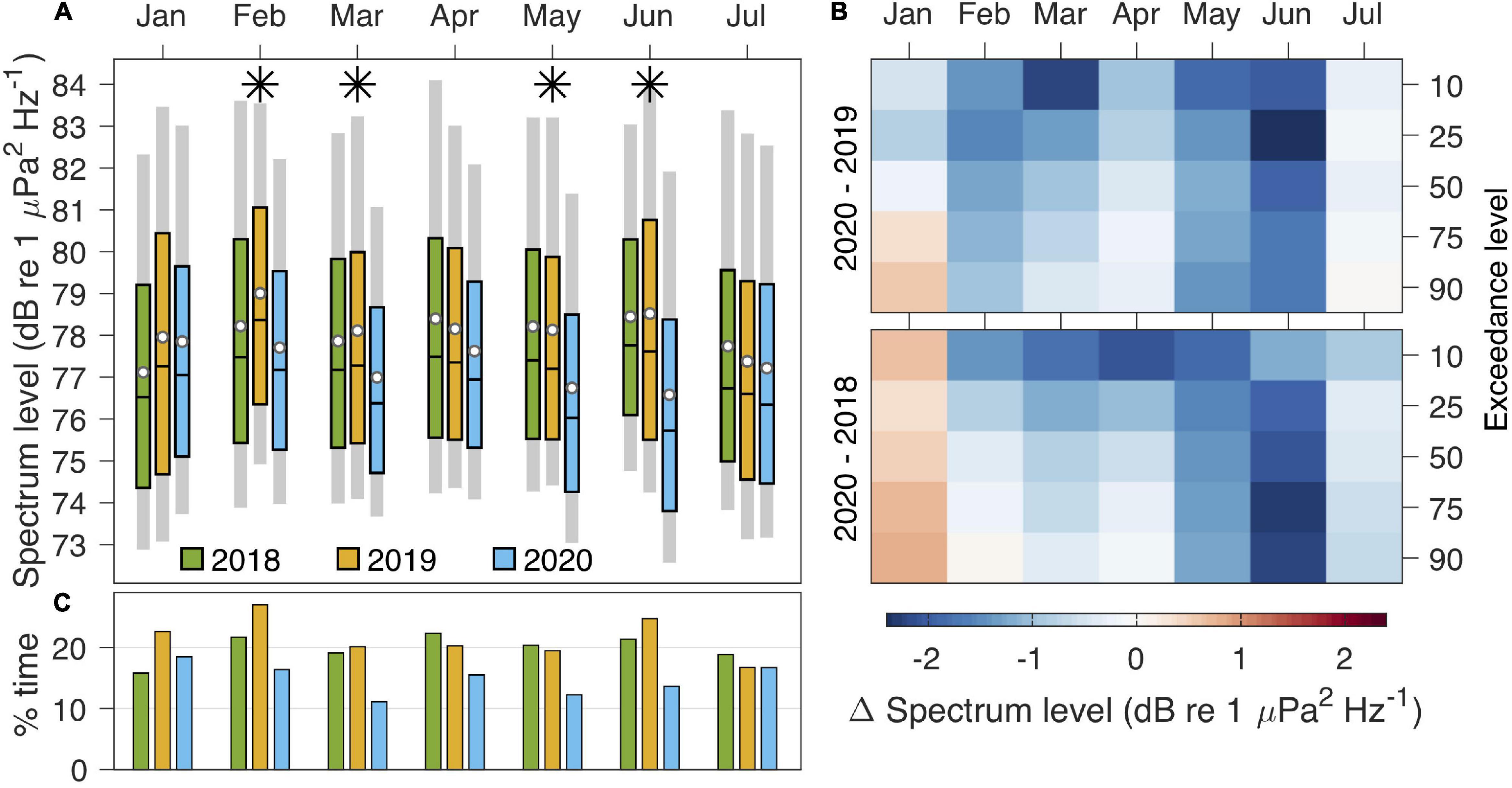
Figure 6. Reduction of low-frequency noise during 2020. (A) Monthly statistics for spectrum levels computed from MARS recordings (location in Figure 1) for a frequency band that is representative of low-frequency vessel noise (one-third octave band centered at 63 Hz, Figure 4). Shown are the range of the 10th–90th exceedance levels (light gray bars), the median and interquartile range (colored boxes), and the geometric mean (white circles). Asterisks indicate months during which spectrum levels were lower during 2020 by at least 1 dB re 1 μPa² Hz^{− 1} relative to at least one of the two preceding years. (B) Percentile-dependent differences between 2020 and the prior 2 years. (C) Monthly percent of time during which 1-min L50 values were more than 3 dB re 1 μPa² Hz^{− 1} above the overall time-series mean.

Low-Frequency Noise

Measured at the same site with the same calibrated instrument, low-frequency noise levels during February through July 2020 were significantly lower (p < 0.01) than they were during the same months of both 2018 and 2019 (Table 1). During 4 months, geometric mean spectrum levels during 2020 were more than 1 dB re 1 μPa² Hz^–1 below those of a previous year. The differences in means and exceedance levels across years indicate that reduced noise during 2020 was persistent during February through June, with January and July being more similar across years (Figures 6A,B). The lowest spectrum levels, in June 2020, were as much as 1.9 (mean) and 2.4 (25% exceedance level) dB re 1 μPa² Hz^–1 below levels of previous years. These changes in central tendency and distribution paralleled reductions in the percent of time during which relatively loud ambient noise (>3 dB above the overall mean) was recorded (Figure 6C).

TABLE 1

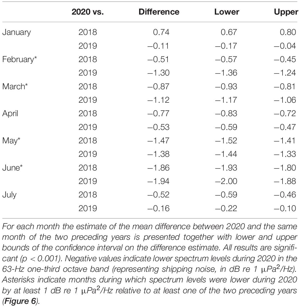
Table 1. Results from Tukey Honest Significant Differences (HSD) multiple comparison applied to ANOVA models fit to data from each month across 2018–2020.

Relationship Between Low-Frequency Noise and Large-Vessel Activity

Shipping total gross tonnage data cover four ports to the north of Monterey Bay and four ports to the south (Figure 7A). During the study period, total gross tonnage across the most- to least-active ports spanned more than three orders of magnitude (Figure 7B). AIS vessel tracking data (Figure 8A), weighted by modeled acoustic transmission loss (Figure 8B) and vessel speed, enable examination of the relationship between shipping and ambient noise within a more regional context.

FIGURE 7

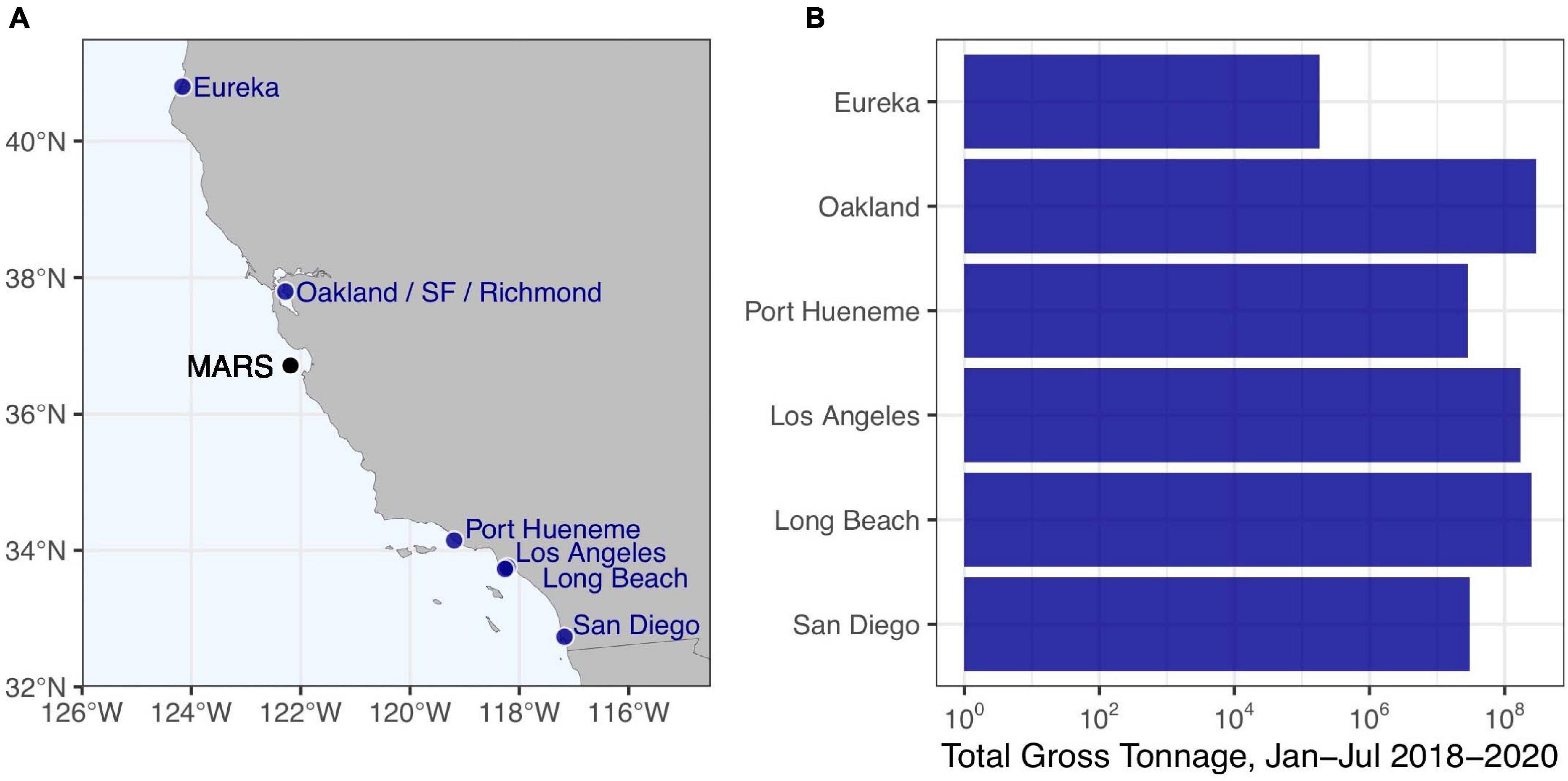
Figure 7. Statewide port activity. (A) Locations of California ports relative to MARS, and (B) total gross tonnage for January through July, 2018 through 2020, the time period for which acoustic data were analyzed (Figure 6). Records for the ports of San Francisco and Richmond are grouped with Oakland; Los Angeles and Long Beach port entry locations nearly coincide.

FIGURE 8

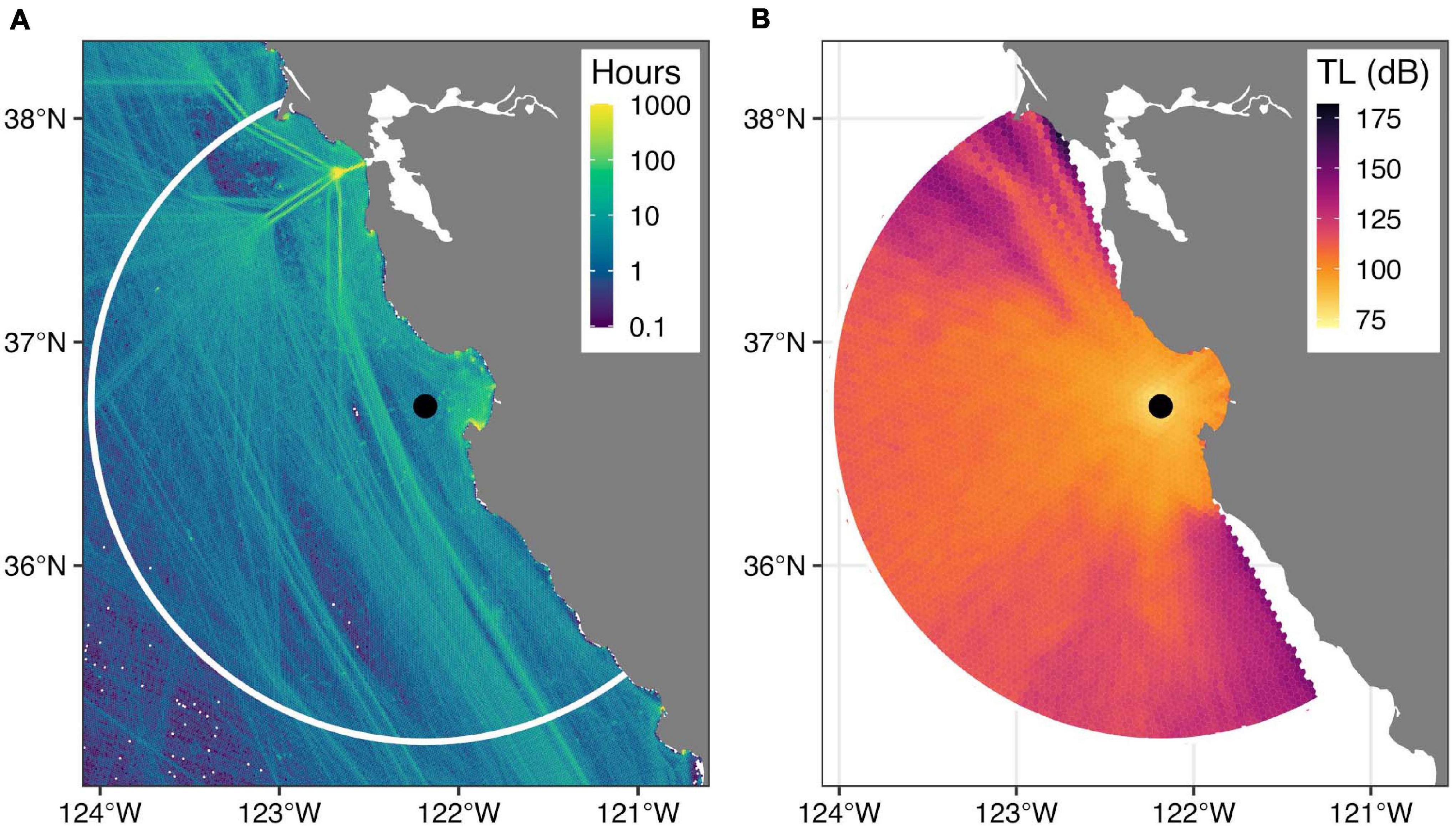
Figure 8. Regional vessel traffic and its weighting. (A) Map of total hours of vessel presence during January through July of 2018–2020, derived from AIS records. Data from within San Francisco Bay were excluded as they would not be relevant to sound recordings at MARS (black circle). (B) Modeled acoustic transmission loss (TL) for a 63 Hz source at 6 m depth (section “Acoustic Modeling”), used as one of two weighting factors for AIS records (section “Automatic Identification System Vessel Tracking Data and Analyses”). The white arc in (A) represents a 165-km radius around MARS, corresponding to the domain of TL modeling in (B).

Variations in low-frequency ambient noise were significantly correlated with both total gross tonnage across all California ports and weighted regional AIS vessel presence (Figure 9 and Table 2). For the AIS metric, the highest adjusted r²-values resulted from inclusion of only the vessel categories having the largest average vessel length: cargo, tanker, other large (USCG ship and cargo types beginning with 9), and enforcement; these comprised 66% of all records within the 165 km radius of MARS. The lowest values of both large-vessel activity and ambient noise occurred during 2020, with the three lowest values during March, May, and June (Figures 6 and 9). Using both port and AIS data across all years, the generalized additive model for the relationship between large-vessel activity and ambient low-frequency noise had an adjusted r² of 0.61. Considered independently, the more regional metric of large-vessel activity (AIS) was the better predictor (Table 2). The relationships between large-vessel activity metrics and ambient noise considering only 2020 were stronger than the overall relationships, with the AIS-based linear model having an adjusted r² of 0.81 (Table 2).

TABLE 2

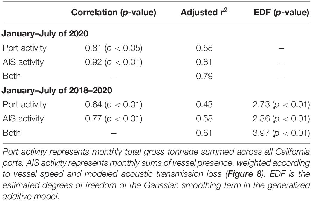
Table 2. Summary of statistical relationships between monthly mean spectrum levels in the 63 Hz one-third octave band and shipping activity metrics (Figure 9).

FIGURE 9

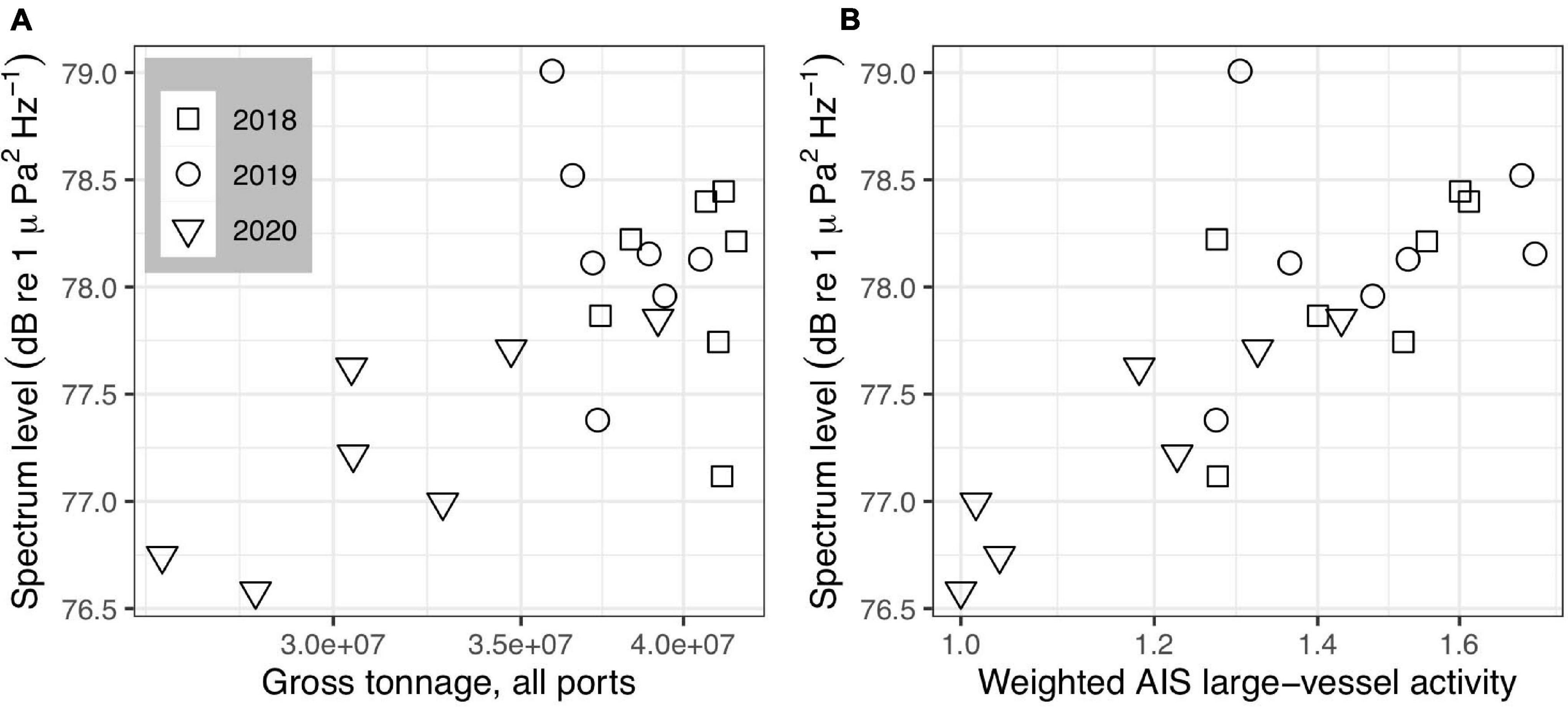
Figure 9. Relationships between metrics of regional large-vessel activity and low-frequency noise at MARS. The low-frequency noise metric is the monthly geometric mean spectrum level for the 63 Hz one-third octave band (Figure 6); both vessel activity metrics are plotted on a logarithmic scale. Metrics of regional large-vessel activity are (A) monthly sums of gross tonnage for California ports (Figure 7), and (B) monthly sums of vessel presence derived from AIS records that were weighted according to modeled acoustic transmission loss (Figure 8) and vessel speed. Monthly sums in (B) are normalized to the minimum to facilitate interpretation. The maximum is ∼ 72% greater than the minimum.

Discussion

COVID-related changes in maritime transportation were directly linked with low-frequency ambient noise within the protected marine habitat of MBNMS. Independent measures of variation in large-vessel activity, based on statewide economic data and regional AIS vessel tracking, were significantly correlated with variation in ambient noise at the MARS recording site. Considering only variations within 2020, the year during which pandemic impacts on shipping activity began to emerge along the U.S. west coast, reduction of low-frequency noise was clearly caused by reduced vessel traffic. Considering variations across 2018–2020, this causal relationship also explains why 2020 ambient noise levels were anomalously low. Acoustic modeling supported the conclusions that the ambient noise measurements represent regional changes in shipping traffic, and that the changes are representative of what animal populations near the recording site would experience.

A previous study off southern California revealed a clear relationship between economic recession, reduced shipping activity, and reduced ambient noise (McKenna et al., 2012). Examining 1 Hz bands centered at 40 and 90 Hz, this earlier study found decreases of 5.1 and 3.1 dB, respectively, between July 2008 and May 2009. Our methods differ from those of this study in a number of ways, including proximity of the recorder to the shipping lanes (distance ∼4X greater in our study), frequency bands used to characterize vessel noise, minimizing error from transient signals, and quantifying change (trend from a continuous data series less than 1 year in length vs. year-to-year comparison of same months across 3 years). Therefore, it is difficult to directly compare results from these studies quantitatively. However, the cause of quieting, traced to economic drivers of maritime shipping, is consistent.

The reduced noise during 2020 relative to preceding years (2018 and 2019) was evident in not only the statistics of central tendency and distribution (mean, percentiles), but also the percentage of time during which relatively loud noise (>3 dB above the mean for the entire study period) was recorded. The consistency of these measures illustrates the cause and effect relationship: less frequent presence of shipping noise caused a decrease in the mean and percentiles for the band that represents this noise source. The nature of this relationship, in turn, frames consideration of consequences. From the perspective of animals that use low-frequency sound to communicate, individual vessel transits would not be quieter, but there would be less time during which vessel noise could mask communication, reduce communication range, or induce stress (Hatch et al., 2012; Erbe et al., 2016, 2019). Evaluation of the consequences of variations in noise exposure requires consideration of both source attributes (spatial, temporal, frequency) and receiver attributes (hearing responses of different species (Southall et al., 2019) and proximity of their populations to noise sources). While direct hearing measurements are lacking for baleen whales for whom changes in low-frequency noise may be most relevant among marine mammals, previous auditory studies have demonstrated that other marine mammal species are able to distinguish between certain sounds with relative differences on the order of 2–3 dB (Moore and Schusterman, 1976; Johnson, 1986).

The ambient noise reduction during 2020 approached the magnitude of decadal increase in low-frequency noise caused by growth in eastern North Pacific shipping activity between the 1950’s and 1990’s (Andrew et al., 2002, 2011; McDonald et al., 2006). Occurring over 5 months (between January and June), this represents a rapid rate of change compared to the decadal trends associated with increased shipping activity in the region. These relative measures of change illustrate the ephemeral nature of noise as an energetic pollutant (Boebel et al., 2018). Noise does not have the degree of persistence that other forms of energetic (heat) or substantial (chemical, plastic, greenhouse gas) pollution have, which offers immediate response to the application of solutions. Collaborations across industry, academia, non-profit, and governmental sectors have great potential to rapidly enhance habitat quality and protection by engineering transitions to a quieter ocean through measures ranging from ship design to speed regulation (McKenna et al., 2013; Southall et al., 2017; Erbe et al., 2019; Chou et al., 2021). This remains an important area of evolving effort in ocean stewardship¹.

Impacts of this global pandemic on ocean soundscapes will vary greatly from region to region, depending on local environmental factors and the type and amount of anthropogenic noise that was typically present before pandemic impacts occurred. Located somewhat near offshore shipping lanes and within MBNMS, the MARS observatory was effective for examining changes in low-frequency noise from large vessels and associated impacts on protected habitat. In considering impacts on marine animals, this study examined frequencies important to baleen whale communication having a high degree of overlap with shipping noise (e.g., Erbe et al., 2019). While these baleen whale species, two of which remain endangered (blue and fin whales), are central to considering impacts of low-frequency noise, it is also important to consider the impacts of this type of noise on other mammals (mysticetes, odontocetes, pinnipeds) that inhabit the sanctuary, as well as fish species that use low-frequency communication (Erbe et al., 2019; Bolgan and Parmentier, 2020; Duarte et al., 2021). Moored recorders have been deployed in other parts of MBNMS, including sites closer to vessel activities of fishing and tourism, and these recordings may enable different insights into the relationships between changes in human activity and acoustic habitat in this marine sanctuary. Soundscape monitoring across U.S. National Marine Sanctuaries (NOAA, 2021) can expand perspective on the acoustic consequences of the pandemic within marine protected areas at the national scale. Global efforts to comprehensively examine changes in ocean soundscapes resulting from the COVID-19 pandemic are ongoing, such as through the International Quiet Ocean Experiment project (Tyack et al., 2021). Advancing our understanding of ocean soundscapes is an essential element of both holistic ecosystem assessment and promotion of ocean health.

Data Availability Statement

The datasets generated and analyzed in this study are available online: https://doi.org/10.6084/m9.figshare.c.5356514.v1. For reproducibility and extensibility of results, original audio recordings for the entire study period, decimated to a sample rate of 2 kHz, are accessible through the AWS Open Data registry: arn:aws:s3:::pacific-sound-2khz.

Author Contributions

JR, JJ, LH, BS, AD, LP, TM, SB-P, and AS contributed to conception and design of the study. JR, JJ, TM, LH, AA, AR, DC, BJ, YZ, and PM contributed to data acquisition, processing, and analysis. JR wrote the first draft of the manuscript. All authors contributed to revision of the original and post-review manuscripts and read and approved the submitted versions.

Funding

The NSF funded installation and maintenance of the MARS cabled observatory through awards 0739828 and 1114794. The SanctSound project, co-led by the US Navy and NOAA, supported collaboration by JR, JJ, LH, AD, TM, BS, LP, SB-P, and AS on this project. Sound recording through the MARS cabled observatory was supported by the Monterey Bay Aquarium Research Institute, with funding from the David and Lucile Packard Foundation.

Conflict of Interest

The authors declare that the research was conducted in the absence of any commercial or financial relationships that could be construed as a potential conflict of interest.

Acknowledgments

We thank C. Dawe, D. French, and the crew of the R/V Rachel Carson for design, deployment, and maintenance of the MARS hydrophone system.

Footnotes

1. ^ https://green-marine.org/certification/scope-and-criteria/underwater-noise-ship-owners/ https://www.portvancouver.com/environmental-protection-at-the-port-of-vancouver/maintaining-healthy-ecosystems-throughout-our-jurisdiction/echo-program/

References

Andrew, R. K., Howe, B. M., and Mercer, J. A. (2011). Long-time trends in ship traffic noise for four sites off the North American West Coast. J. Acoust. Soc. Am. 129:642. doi: 10.1121/1.3518770

CrossRef Full Text | Google Scholar

Andrew, R. K., Howe, B. M., Mercer, J. A., and Dzieciuch, M. A. (2002). Ocean ambient sound: comparing the 1960s with the 1990s for a receiver off the California coast. ARLO 3, 65–70. doi: 10.1121/1.1461915

CrossRef Full Text | Google Scholar

Boebel, O., Burkhardt, E., and van Opzeeland, I. (2018). “Input of energy/underwater noise,” in Handbook on Marine Environment Protection, eds M. Salomon and T. Markus, (Berlin: Springer), 1024. doi: 10.1007/978-3-319-60156-4.

CrossRef Full Text | Google Scholar

Bolgan, M., and Parmentier, E. (2020). The unexploited potential of listening to deep-sea fish. Fish Fish. 21, 1238–1252. doi: 10.1111/faf.12493

CrossRef Full Text | Google Scholar

Calambokidis, J., Steiger, G. H., Curtice, C., Harrison, J., Ferguson, M. C., Becker, E. A., et al. (2015). Biologically important areas for selected cetaceans within U.S. waters – West Coast region. Aquat. Mamm. 41, 39–53. doi: 10.1578/AM.41.1.2015.39

CrossRef Full Text | Google Scholar

Chou, E., Southall, B. L., Robards, M., and Rosenbaum, H. C. (2021). International policy, recommendations, actions and mitigation efforts of anthropogenic underwater noise. Ocean Coast. Manag. 202:105427. doi: 10.1016/j.ocecoaman.2020.105427

CrossRef Full Text | Google Scholar

Collins, M. D. (1993). A split-step Padé solution for the parabolic equation method. J. Acoust. Soc. Am. 93, 1736–1742. doi: 10.1121/1.406739

CrossRef Full Text | Google Scholar

Dahlheim, M., and Castellote, M. (2016). Changes in the acoustic behavior of gray whales Eschrichtius robustus in response to noise. Endanger. Species Res. 31, 227–242. doi: 10.3354/esr00759

CrossRef Full Text | Google Scholar

Dekeling, R. P. A., Tasker, M. L., Van der Graaf, A. J., Ainslie, M. A., Andersson, M. H., Andreì, M., et al. (2014). Monitoring Guidance for Underwater Noise in European Seas, Part II: Monitoring Guidance Specifications, JRC Scientific and Policy Report EUR 26555 EN. Luxembourg: Publications Office of the European Union.

Google Scholar

Duarte, C. M., Chapuis, L., Collin, S. P., Costa, D. P., Devassy, R. P., Eguiluz, V. M., et al. (2021). The soundscape of the Anthropocene ocean. Science 371:eaba4658. doi: 10.1126/science.aba4658

PubMed Abstract | CrossRef Full Text | Google Scholar

Ekstrom, J. A. (2009). California current large marine ecosystem: publicly available dataset of state and federal laws and regulations. Mar. Policy 33, 528–531. doi: 10.1016/j.marpol.2008.11.002

CrossRef Full Text | Google Scholar

Erbe, C., Marley, S. A., Schoeman, R. P., Smith, J. N., Trigg, L. E., and Embling, C. B. (2019). The effects of ship noise on marine mammals—a review. Front. Mar. Sci. 6:606. doi: 10.3389/fmars.2019.00606

CrossRef Full Text | Google Scholar

Erbe, C., Reichmuth, C., Cunningham, K., Lucke, K., and Dooling, R. (2016). Communication masking in marine mammals: a review and research strategy. Mar. Poll. Bull. 103, 15–38. doi: 10.1016/j.marpolbul.2015.12.007

PubMed Abstract | CrossRef Full Text | Google Scholar

Gedamke, J., Harrison, J., Hatch, L., Angliss, R., Barlow, J., Berchok, C., et al. (2016). NOAA Ocean Noise Strategy Roadmap. Washington, DC: NOAA, 138.

Google Scholar

Goley, P. D., and Straley, J. M. (1994). Attack on gray whales (Eschrichtius robustus) in Monterey Bay, California, by killer whales (Orcinus orca) previously identified in Glacier Bay, Alaska. Can. J. Zool. 72, 1528–1530. doi: 10.1139/z94-202

CrossRef Full Text | Google Scholar

Gottesman, B. L., Sprague, J., Kushner, D. J., Bellisario, K., Savage, D., McKenna, M. F., et al. (2020). Soundscapes indicate kelp forest condition. Mar. Ecol. Prog. Ser. 654, 35–52. doi: 10.3354/meps13512

CrossRef Full Text | Google Scholar

Hatch, L., Clark, C., Merrick, R., Van Parijs, S., Ponirakis, D., Schwehr, K., et al. (2008). Characterizing the relative contributions of large vessels to total ocean noise fields: a case study using the Gerry E. Studds Stellwagen Bank National Marine Sanctuary. Environ. Manage. 42, 735–752. doi: 10.1007/s00267-008-9169-4

PubMed Abstract | CrossRef Full Text | Google Scholar

Hatch, L. T., Clark, C. W., Van Parijs, S. M., Frankel, A. S., and Ponirakis, D. W. (2012). Quantifying loss of acoustic communication space for right whales in and around a U.S. National Marine Sanctuary. Conserv. Biol. 26, 983–994. doi: 10.1111/j.1523-1739.2012.01908.x

PubMed Abstract | CrossRef Full Text | Google Scholar

Hatch, L. T., Wahle, C. M., Gedamke, J., Harrison, J., Laws, B., Moore, S. E., et al. (2016). Can you hear me here? Managing acoustic habitat in US waters. Endang. Species Res. 30, 171–186. doi: 10.3354/esr00722

CrossRef Full Text | Google Scholar

Helble, T. A., Guazzo, R. A., Alongi, G. C., Martin, C. R., Martin, S. W., and Henderson, E. E. (2020). Fin whale song patterns shift over time in the Central North Pacific. Front. Mar. Sci. 7:907. doi: 10.3389/fmars.2020.587110

CrossRef Full Text | Google Scholar

Hildebrand, J. A. (2009). Anthropogenic and natural sources of ambient noise in the ocean. Mar. Ecol. Prog. Ser. 395, 5–20. doi: 10.3354/meps08353

CrossRef Full Text | Google Scholar

IQOE, (2019). IQOE Workshop Report: Guidelines for Observation of Ocean Sound. St. Petersburg, FL: IQOE.

Google Scholar

ISO, (2017). International Standard ISO 18405:2017(E), Underwater Acoustics – Terminology. Geneva: ISO.

Google Scholar

Johnson, C. S. (1986). “Dolphin audition and echolocation capacities,” in Dolphin Cognition and Behavior: A Comparative Approach, eds R. J. Schusterman, J. A. Thomas, F. G. Wood, and R. Schusterman, (Boca Raton, FL: CRC Press), 115–136.

Google Scholar

Kline, L. R., DeAngelis, A. I., McBride, C., Rodgers, G. G., Rowell, T. J., Smith, J., et al. (2020). Sleuthing with sound: understanding vessel activity in marine protected areas using passive acoustic monitoring. Mar. Policy 120:104138. doi: 10.1016/j.marpol.2020.104138

CrossRef Full Text | Google Scholar

McDonald, M. A., Hildebrand, J. A., and Wiggins, S. M. (2006). Increases in deep ocean ambient noise in the Northeast Pacific west of San Nicolas Island, California. J. Acoust. Soc. Am. 120:711. doi: 10.1121/1.2216565

CrossRef Full Text | Google Scholar

McKenna, M. F., Katz, S. L., Wiggins, S. M., Ross, D., and Hildebrand, J. A. (2012). A quieting ocean: unintended consequence of a fluctuating economy. J. Acoust. Soc. Am. 132, EL169–EL175. doi: 10.1121/1.4740225

CrossRef Full Text | Google Scholar

McKenna, M. F., Wiggins, S. M., and Hildebrand, J. A. (2013). Relationship between container ship underwater noise levels and ship design, operational and oceanographic conditions. Sci. Rep. 3:1760. doi: 10.1038/srep01760

CrossRef Full Text | Google Scholar

Moore, P. W., and Schusterman, R. J. (1976). Discrimination of pure-tone intensities by the California sea lion. J. Acoust. Soc. Am. 60, 1405–1407. doi: 10.1121/1.381234

CrossRef Full Text | Google Scholar

NOAA, (2017). Marine Mammals: MBNMS. Washington, DC: NOAA.

Google Scholar

NOAA, (2021). Sound Monitoring. Washington, DC: NOAA.

Google Scholar

Oestreich, W. K., Fahlbusch, J. A., Cade, D. E., Calambokidis, J., Margolina, T., Joseph, J., et al. (2020). Animal-borne metrics enable acoustic detection of blue whale migration. Curr. Biol. 30, 4773–4779. doi: 10.1016/j.cub.2020.08.105

PubMed Abstract | CrossRef Full Text | Google Scholar

Porter, M. B. (2011). The BELLHOP Manual and User’s Guide: PRELIMINARY DRAFT. La Jolla, CA: Heat Light and Sound Research Inc.

Google Scholar

Rolland, R. M., Parks, S. E., Hunt, K. E., Castellote, M., Corkeron, P. J., Nowacek, D. P., et al. (2012). Evidence that ship noise increases stress in right whales. Proc. Biol. Sci. 279, 2363–2368. doi: 10.1098/rspb.2011.2429

PubMed Abstract | CrossRef Full Text | Google Scholar

Ryan, J., Cline, D., Dawe, C., McGill, P., Zhang, Y., Joseph, J., et al. (2016). “New passive acoustic monitoring in Monterey Bay National Marine Sanctuary,” in Proceedings of the OCEANS 2016 MTS/IEEE Monterey (Monterey, CA: IEEE), 1–8 doi: 10.1016/s0025-3227(01)00258-4

CrossRef Full Text | Google Scholar

Ryan, J. P., Cline, D. E., Joseph, J. E., Margolina, T., Santora, J. A., Kudela, R. M., et al. (2019). Humpback whale song occurrence reflects ecosystem variability in feeding and migratory habitat of the northeast Pacific. PLoS One 14:e0222456. doi: 10.1371/journal.pone.0222456

PubMed Abstract | CrossRef Full Text | Google Scholar

Simonis, A. E., Brownell, R. L., Thayre, B. J., Trickey, J. S., Oleson, E. M., Huntington, R., et al. (2020a). Co-occurrence of beaked whale strandings and naval sonar in the Mariana Islands, Western Pacific. Proc. Biol. Sci. 287:20200070. doi: 10.1098/rspb.2020.0070

PubMed Abstract | CrossRef Full Text | Google Scholar

Simonis, A. E., Forney, K. A., Rankin, S., Ryan, J., Zhang, Y., DeVogelaere, A., et al. (2020b). Seal bomb noise as a potential threat to Monterey Bay Harbor porpoise. Front. Mar. Sci. 7:142. doi: 10.3389/fmars.2020.00142

CrossRef Full Text | Google Scholar

Southall, B., Berkson, J., Bowen, D., Brake, R., Eckman, J., Field, J., et al. (2009). Addressing the Effects of Human-Generated Sound on Marine Life: An Integrated Research Plan for U.S. Federal Agencies, Interagency Task Force on Anthropogenic Sound and the Marine Environment of the Joint Subcommittee on Ocean Science and Technology. Washington, DC: Marine Mammal Commission.

Google Scholar

Southall, B. L., Finneran, J. J., Reichmuth, C., Nachtigall, P. E., Ketten, D. R., Bowles, A. E., et al. (2019). Marine mammal noise exposure criteria: updated scientific recommendations for residual hearing effects. Aquat. Mamm. 45, 125–232. doi: 10.1578/AM.45.2.2019.125

CrossRef Full Text | Google Scholar

Southall, B. L., Scholik-Schlomer, A. R., Hatch, L., Bergmann, T., Jasny, M., Metcalf, K., et al. (2017). Underwater Noise from Large Commercial Ships—International Collaboration for Noise Reduction. Encyclopedia of Maritime and Offshore Engineering. Hoboken, NJ: John Wiley & Sons, Ltd. doi: 10.1002/9781118476406.emoe056

CrossRef Full Text | Google Scholar

Thomson, D. J. M., and Barclay, D. R. (2020). Real-time observations of the impact of COVID-19 on underwater noise. J. Acoust. Soc. Am. 147:3390. doi: 10.1121/10.0001271

CrossRef Full Text | Google Scholar

Tyack, P. L., Miksis-Olds, J., Ausubel, J., and Urban, E. R. Jr. (2021). Measuring Ambient Ocean Sound During the COVID-19 Pandemic. Livonia, MI: EOS, 102

Google Scholar

USCG, (2021). Navigation Center, United States Coast Guard. Available online at: https://www.navcen.uscg.gov/?pageName=AISMessagesAStatic#TypeOfShip (accessed November 1, 2020).

Google Scholar

Wenz, G. M. (1962). Acoustic ambient noise in the ocean: spectra and sources. J. Acoust. Soc. Am. 34, 1936–1956. doi: 10.1121/1.1909155

CrossRef Full Text | Google Scholar

Zuur, A. F., and Ieno, E. N. (2016). A protocol for conducting and presenting results of regression-type analyses. Methods Ecol. Evol. 7, 636–645. doi: 10.1111/2041-210X.12577

CrossRef Full Text | Google Scholar